Project 5: Neural Radiance Fields

Part 1: Fit a Neural Field to a 2D Image

To fit a Neural Field to a 2D image, I construct an MLP with the following architecture:

For positional encodings, I use the sine/cosine encodings from the NERF paper with L=10. The full input is a (10*2 + 1)*2 = 42 dimensional vector. I train the network with a learning rate of .01 and a batch size of 10000 for 3000 epochs.

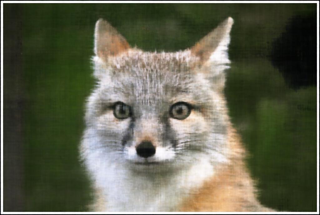
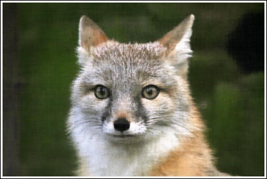
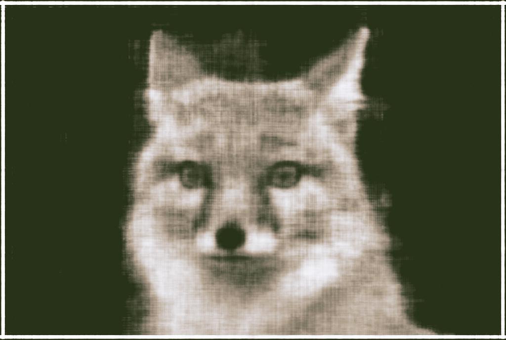
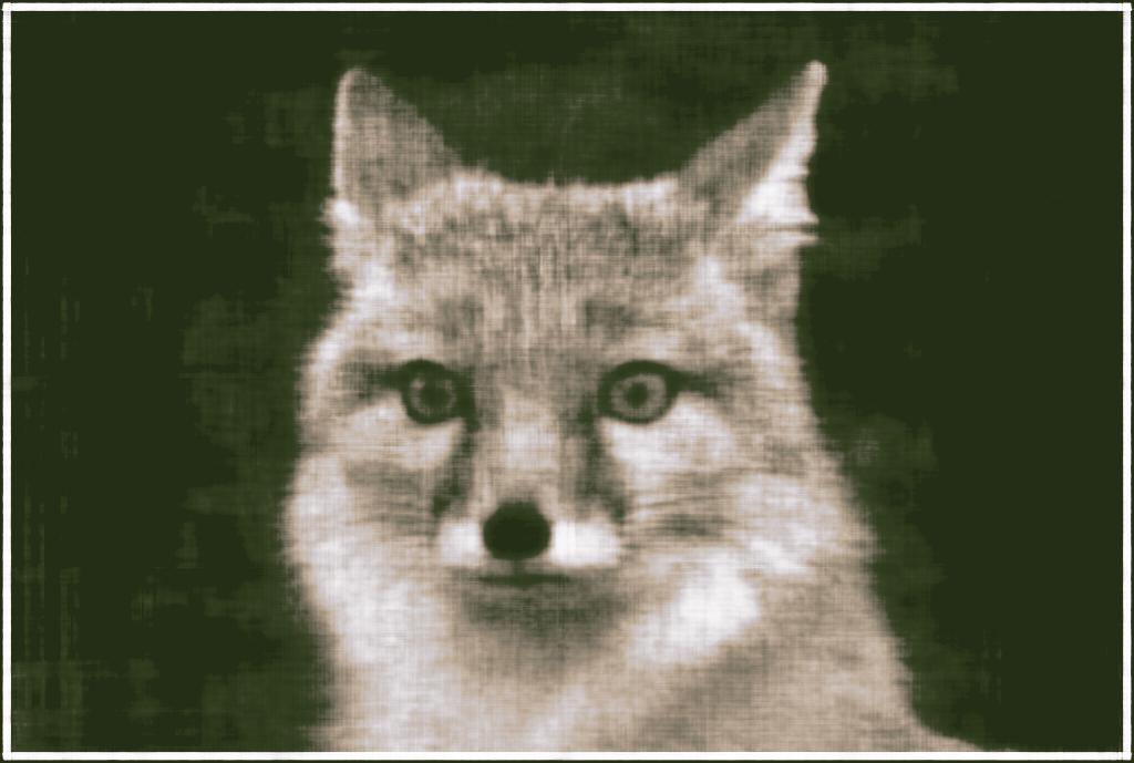
L = 10 Results

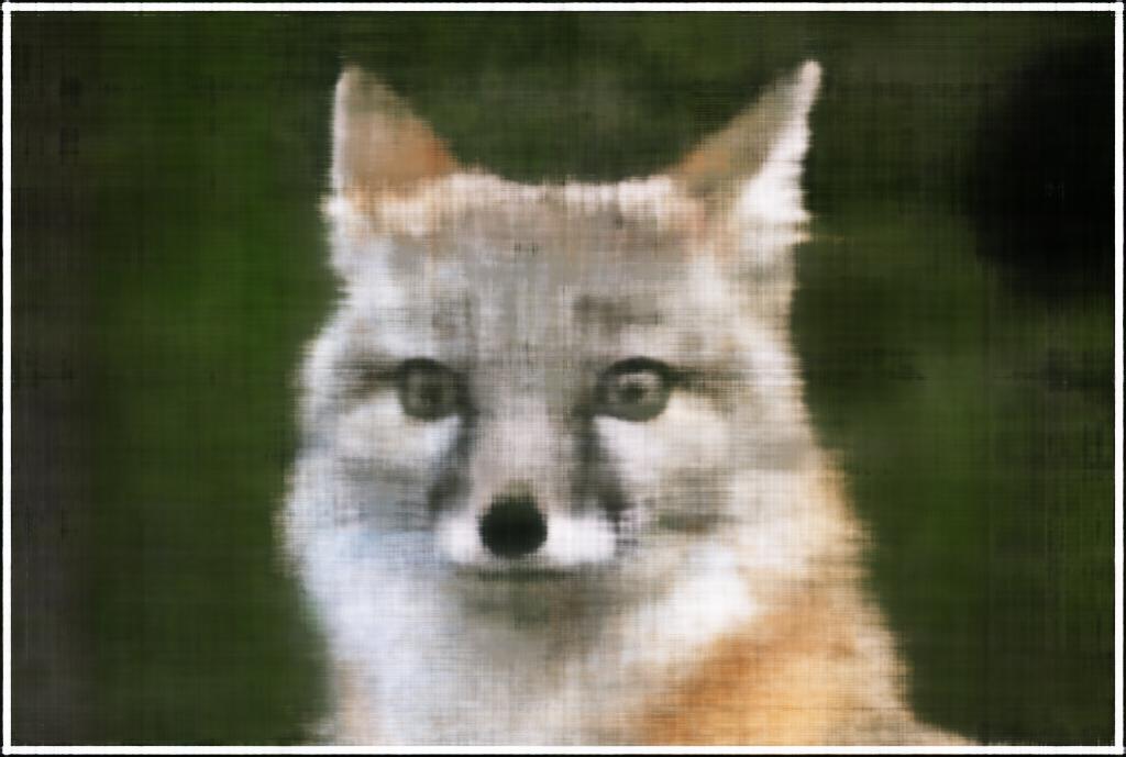
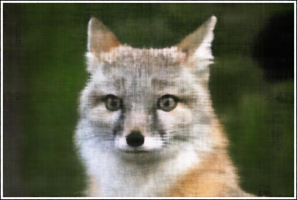
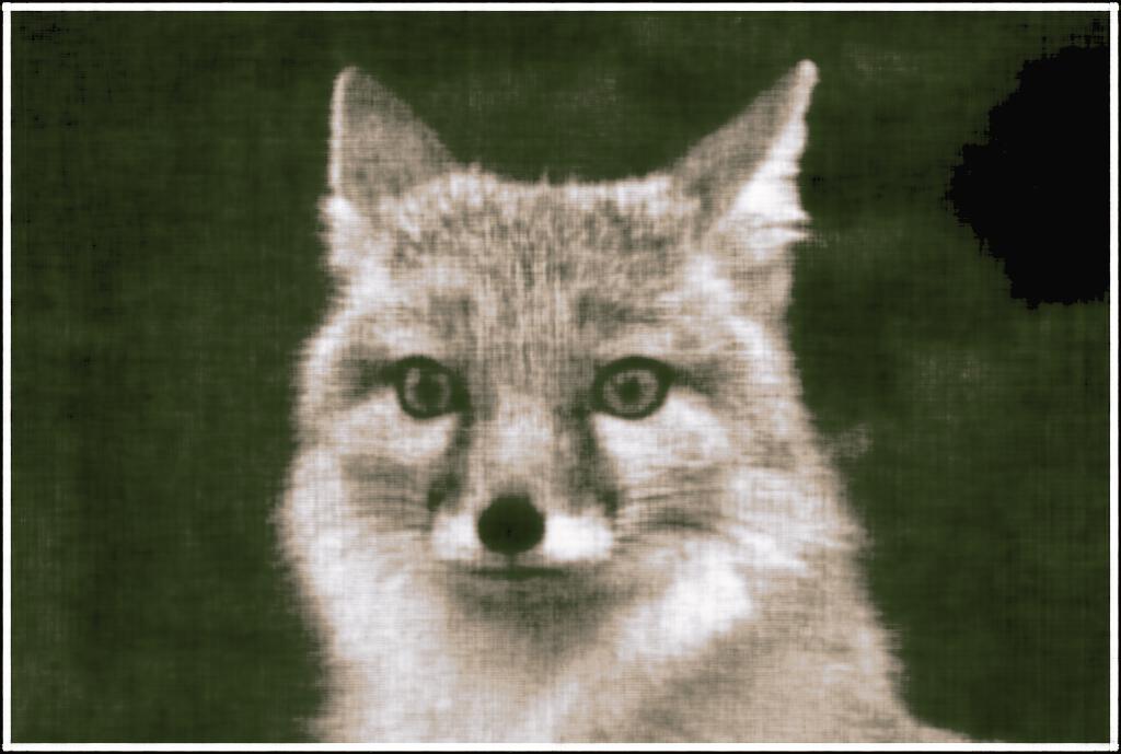
These are the best results. With L=10 and the network as described above, the reconstructed fox is in sharp focus.

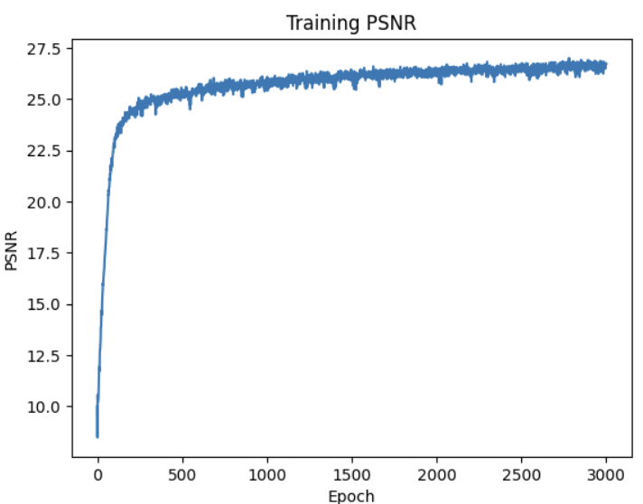
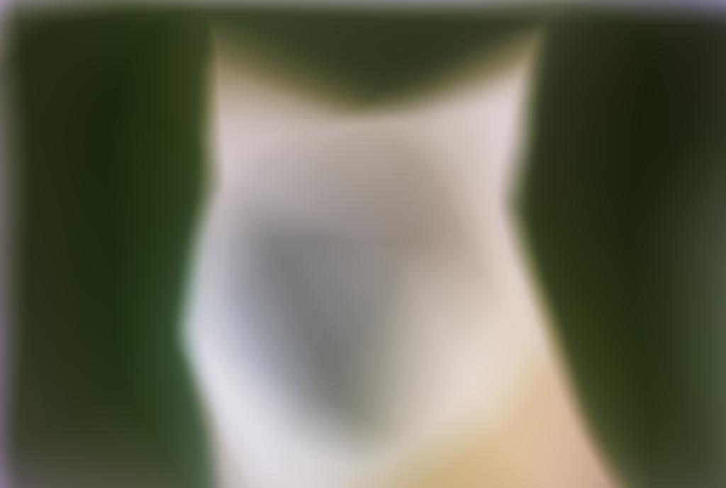
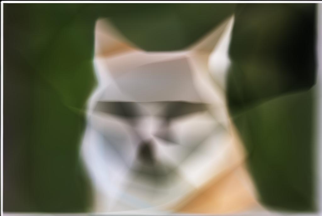
L = 0 Results

With L = 0, there are no positional encodings. The network has a lot of trouble figuring out the geometry of the image, and reconstructing finer features that require small edges.

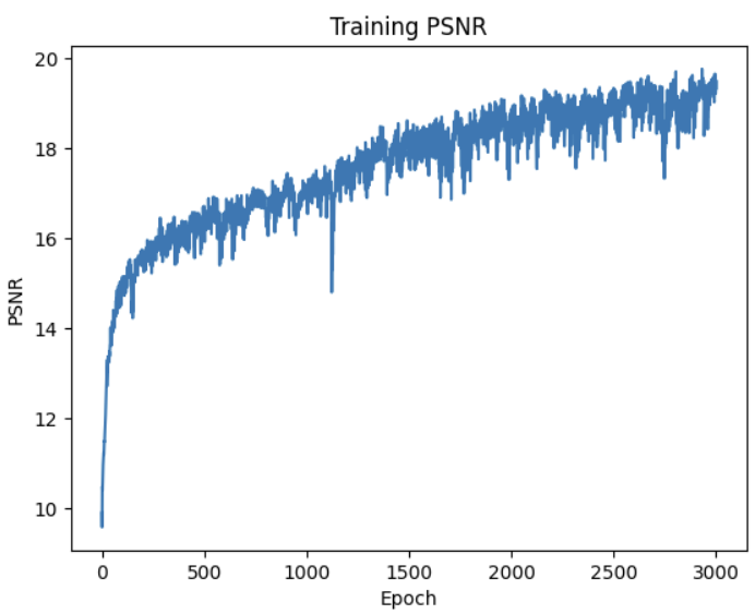
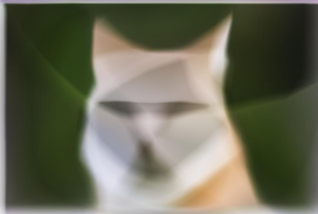
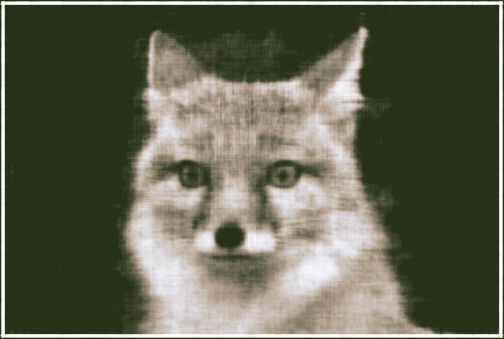
L = 10 with 2 extra hidden layers Results

Curiously, the deeper network has more trouble learning color, but learns the shape of the fox quickly.

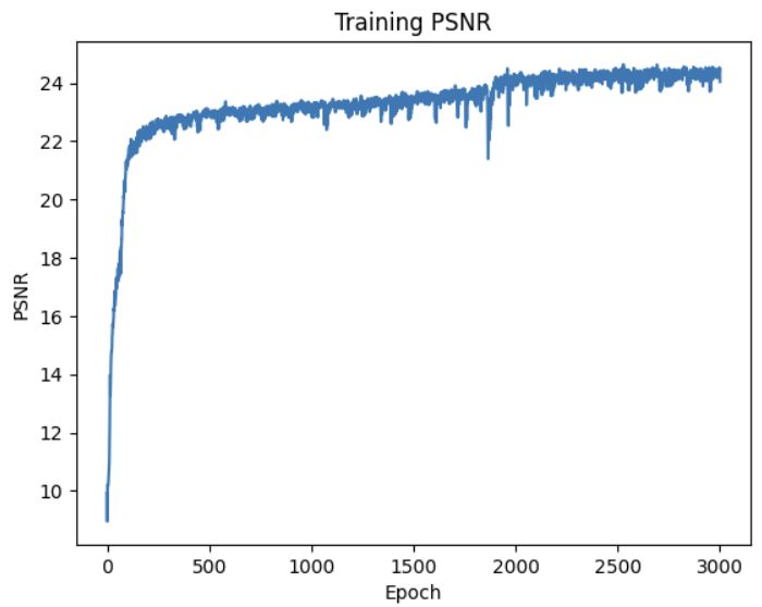
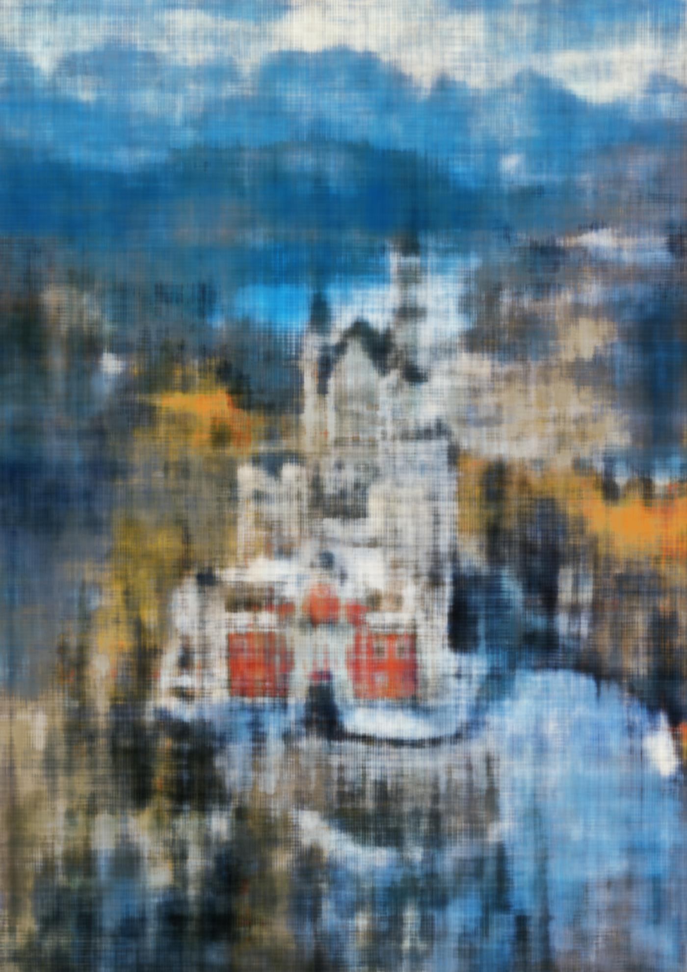
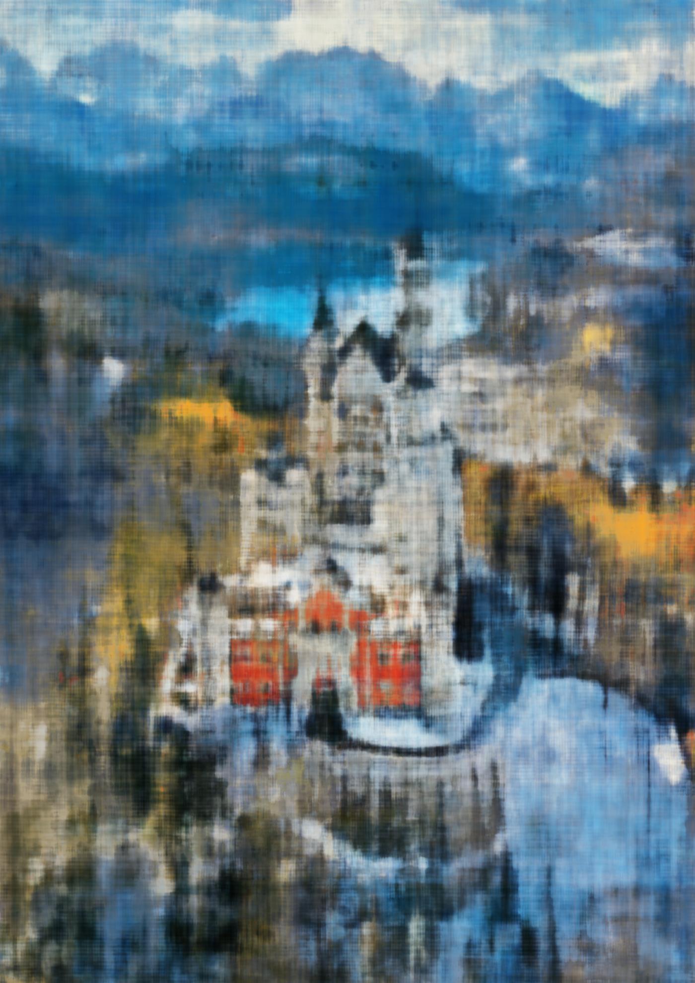
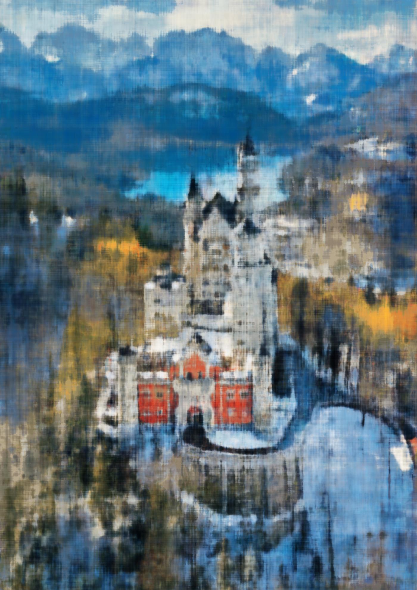
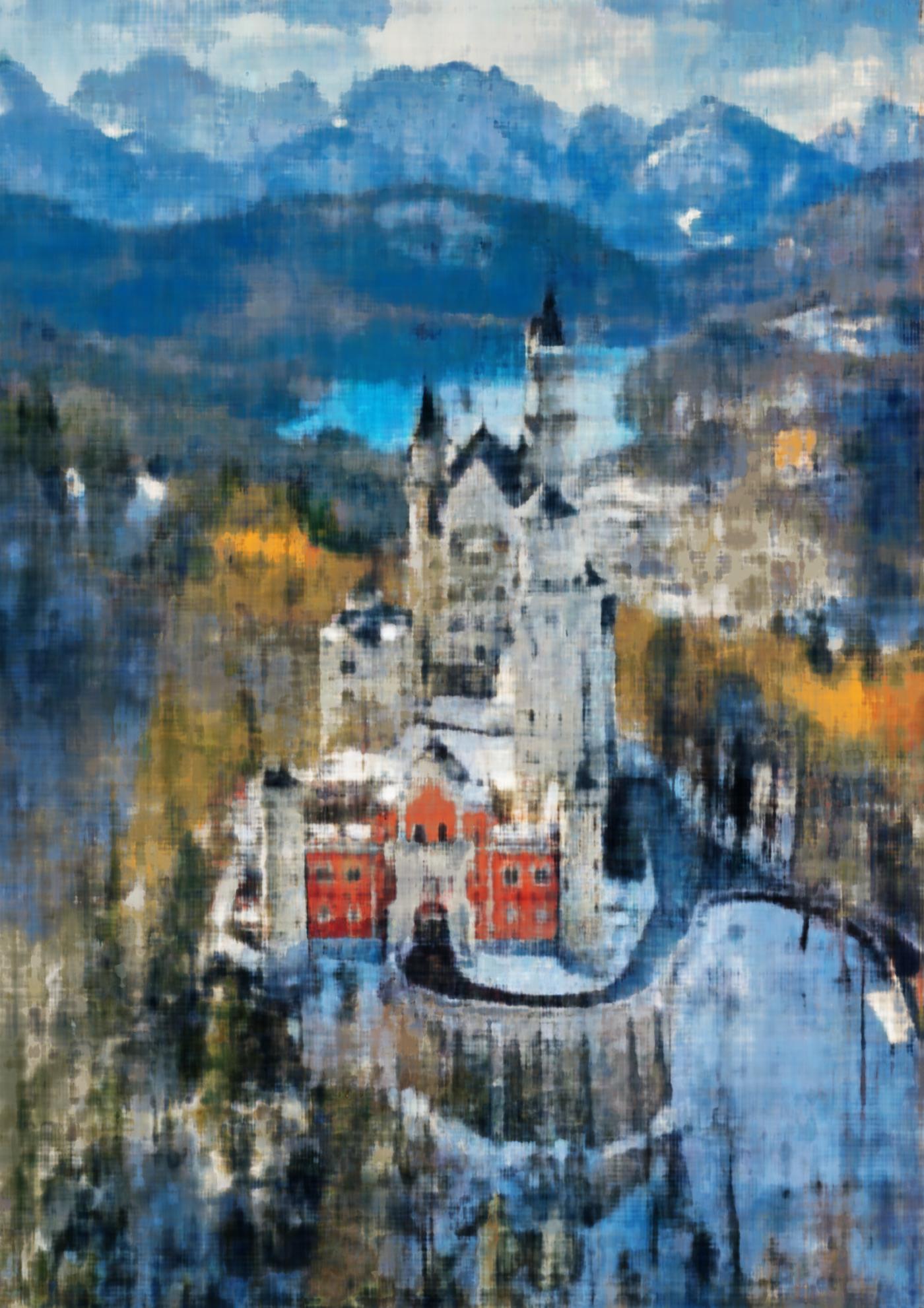
L= 10 on Neuschwanstein

Neuschwanstein is a much harder task to memorize because it is filled with intricate details. However, this network still achieves a reasonable reconstruction of the image.
Original:

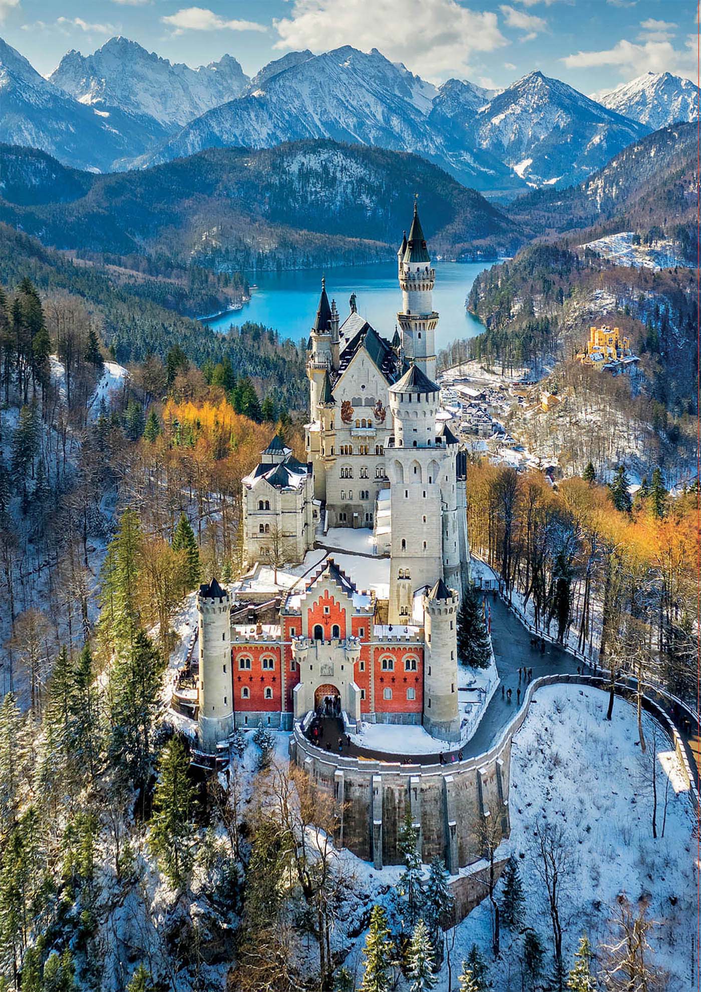Reconstruction training:

Part 2: Fit a Neural Radiance Field from Multi-view Images

Part 2.1: Create Rays from Cameras

Before creating the NERFS, some machinery is needed to convert coordinates. To convert from world to camera coordinates, we define a rotation and translation matrix: \begin{align} \begin{bmatrix} x_c \\ y_c \\ z_c \\ 1 \end{bmatrix} = \begin{bmatrix} \mathbf{R}_{3\times3} & \mathbf{t} \\ \mathbf{0}_{1\times3} & 1 \end{bmatrix} \begin{bmatrix} x_w \\ y_w \\ z_w \\ 1 \end{bmatrix} \end{align} To invert this transformation and convert from camera to world (c2w), I multiply the inverse of the extrinsic matrix by the camera coordinates. \begin{align} \begin{bmatrix} x_w \\ y_w \\ z_w \\ 1 \end{bmatrix} = \begin{bmatrix} \mathbf{R}_{3\times3} & \mathbf{t} \\ \mathbf{0}_{1\times3} & 1 \end{bmatrix}^{-1} \begin{bmatrix} x_c \\ y_c \\ z_c \\ 1 \end{bmatrix} \end{align} To convert from camera coordinates to pixels, we first define the intrinsics matrix: \begin{align} \mathbf{K} = \begin{bmatrix} f_x & 0 & o_x \\ 0 & f_y & o_y \\ 0 & 0 & 1 \end{bmatrix} \end{align} which converts between the coordinate systems as follows: \begin{align} s \begin{bmatrix} u \\ v \\ 1 \end{bmatrix} = \mathbf{K} \begin{bmatrix} x_c \\ y_c \\ z_c \end{bmatrix} \end{align} To convert from pixels to camera coodinates: \begin{align} \mathbf{K}^{-1} s \begin{bmatrix} u \\ v \\ 1 \end{bmatrix} = \begin{bmatrix} x_c \\ y_c \\ z_c \end{bmatrix} \end{align} To convert from pixels to rays, we need to determine the camera location and the direction of the ray. To calculate the camera location from the c2w matrix: \begin{align} \mathbf{r}_o = -\mathbf{R}_{3\times3}^{-1}\mathbf{t} \\ \mathbf{r}_o = \begin{bmatrix} \mathbf{R}_{3\times3} & \mathbf{t} \\ \mathbf{0}_{1\times3} & 1 \end{bmatrix}^{-1} \begin{bmatrix} 0 \\ 0 \\ 0 \\ 1 \end{bmatrix} \end{align} The normalized ray direction is then calculated: \begin{align} \mathbf{r}_d = \frac{\mathbf{X_w} - \mathbf{r}_o}{||\mathbf{X_w} - \mathbf{r}_o||_2} \end{align} I use the previously defined functions to convert from pixel coordinates to camera coordinates, and then from camera coordinates to world coordinates.

Part 2.2: Sampling

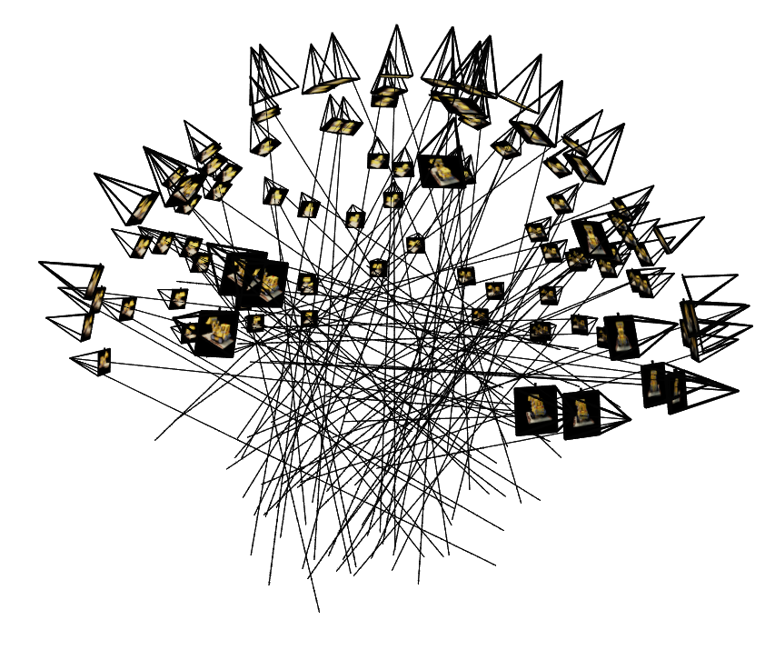
To sample rays for training, I randomly select pixels from all of the training images, and compute the rays that correspond to each. To sample along the ray, I take 32 evenly spaced points between 2.0 and 6.0 units away from the start of the ray. During training, I randomly perturb these samples to be anywhere within the small interval around them. This helps avoid aliasing.

Part 2.3: Putting the Dataloading All Together

Part 2.4: Neural Radiance Field

I use the following architecture for training NERFs. In the 3D setting, we input both the direction of the ray and the coordinates of the points along the ray that we are querying. The NERF then outputs a density and an rgb for each point. The coordinates of the points along the ray, x, are positionally encoded with L=10. The ray directions themselves are also positionally encoded with L=4.

Part 2.5: Volume Rendering

To render the pixel, I use the discrete volume rendering equation: \begin{align} \hat{C}(\mathbf{r})=\sum_{i=1}^N T_i\left(1-\exp \left(-\sigma_i \delta_i\right)\right) \mathbf{c}_i, \text { where } T_i=\exp \left(-\sum_{j=1}^{i-1} \sigma_j \delta_j\right) \end{align} Where \(T_i\) is the transmittance, \(\sigma_j\) is the density, \(\delta_j\) is the sample interval, and \(\mathbf{c}_i\) is the color at this point. During training, I first sample a set of rays, sample points along those rays, and feed this data through the network. The network returns densities and rgbs, so I use the above volume rendering equation to calculate the predicted pixel color. This is then supervised using MSE loss. 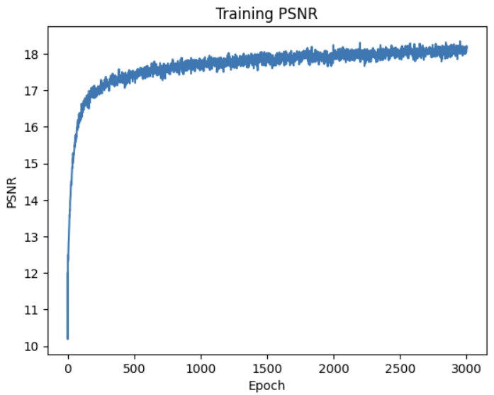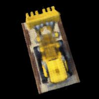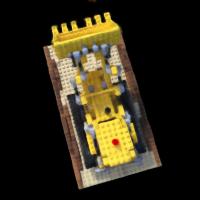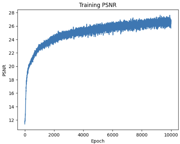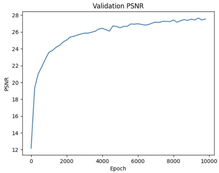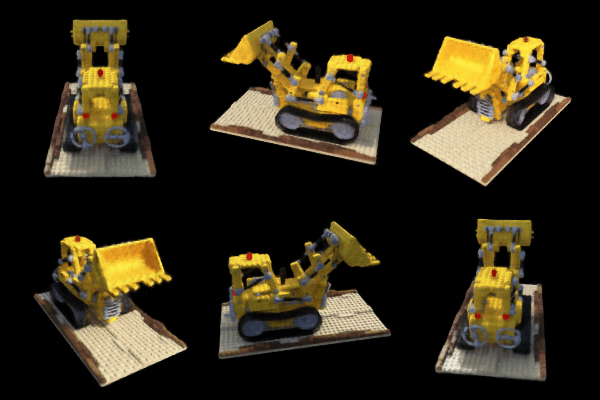Batch size is 10000 and learning rate is .0005 with the Adam optimizer. The below results were trained for 10,000 epochs.

Bells and Whistles

Depth Rendering

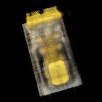
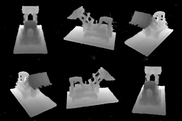
It is possible to extract a depth map of the scene from the trained NERF. To do this, I modify the volume rendering equation to be: \begin{align} \hat{C}(\mathbf{r})=\sum_{i=1}^N T_i\left(1-\exp \left(-\sigma_i \delta_i\right)\right) \mathbf{d}_i, \text { where } \mathbf{d}_i=\sum_{j=1}^{i-1} \delta_j \end{align} Where \(\mathbf{d}_i\) is the distance along the ray. I then normalize the colors to be between 0 and 1.

Changing Background Color

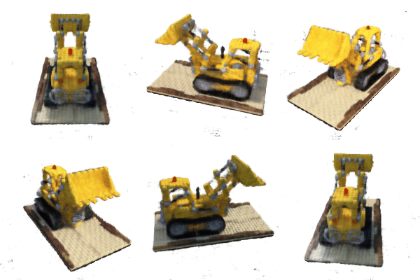
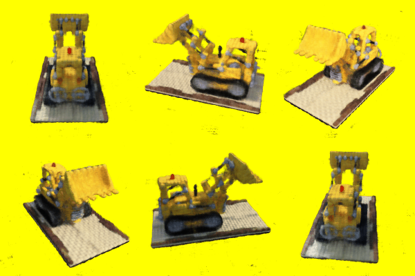
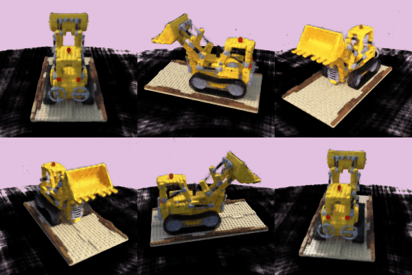
It is also possible to change the background color of the rendered images by modifying the volrend function. To do so, I add modify \(C_r\) as follows: \begin{align} \hat{C}^{'}(\mathbf{r}) = \hat{C}(\mathbf{r}) + T_{N+1}\cdot \mathbf{c_{bg}} \end{align} \(\mathbf{c_{bg}}\) represents the chosen background color, and \(T_{N+1}\) is the probability of the ray not terminating at any of the sample points along the ray, in which case it hits the background. 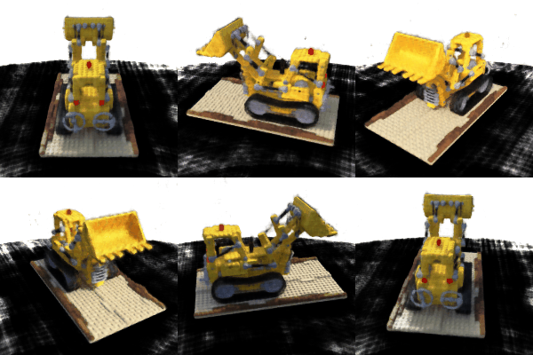Here is the scene with various colored backgrounds after 3000 epochs.

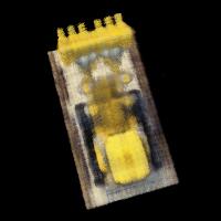
One quirk I noticed during training was that, past a certain point (around 5000 epochs), the NERF began to learn a black floor beneath the truck. This is apparent when the background is rendered to a different color: